Neural Radiance Fields (NeRFS): A Breakdown

In our machine learning courses, much of the content gets broken down based on different types of data. This is sensible – choice of modality goes a long way in determining which methods are relevant. The typical favorites of images and text rightfully attract the bulk of the attention, but along with these staples I personally find something particularly intriguing about data which inhabits 3 dimensions. In all likelihood this is probably a bit self-centered as that’s where I happen to live as well. Given that, it’s been an exciting few years for me as I’ve gotten to witness plenty of progress in this domain, resulting in all sorts of fascinating applications.

In this post, I’d like to give an overview of the methodology which has inspired and enabled much of this recent progress. Neural Radiance Fields (or NeRFs) were first introduced in 2020 and quickly upended the general consensus of what’s possible in 3D machine learning. This is due to their uncanny ability to represent 3D shapes, allowing practitioners to get accurate 3D models just from observations. That same representational capacity can also be applied toward generating novel 3D content for use in virtual applications like animation, video games, VR/AR (“spatial computing” if you’re trendy) or brought into the real world through 3D-printing and AI-powered manufacturing.

My goal is to give a technical understanding of how NeRFs operate, aimed at those who have some basic knowledge of machine learning and neural networks. I’ll also try to motivate this, mainly relying on two applications of NeRFs as examples. The first is 3D reconstruction which is a natural choice since this is sort of the canonical task for NeRFs that spurred their development. The second application is in text-to-3D which I think hints at what a general-purpose representation NeRFs can be and gives a look at a newer area where rapid progress is still ongoing. Regardless, it’s not the specific application that matters here as much as the underlying foundation which allows us to define a fast, flexible, and efficient method for representing 3-dimensional data.

Note: The terms “scene” and “shape” get used interchangeably throughout this post as the unit for a single instance of 3D data. It doesn’t really matter which is used and anything said about one applies equally to the other.

3D Representations

A commensense way of representing 3D content would be to extend the method we use for 2D images and discretize the content into a 3-dimensional grid in $\mathbb{R}^{ N \times N \times N \times 4}$. Here, each voxel would store four values: The RGB color value for the associated region as well as the opacity at this point. Opacity is a value between $0$ and $1$ which essentially just indicates whether something solid (i.e can’t be seen through) is located there. By storing just these four numbers in each location we are able to represent the scene’s radiance properties, which determine how it reflects light and therefore how it will appear when viewed from any angle.

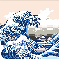
The only loss of information here is going to be due to the discretization as we’re using a fixed resolution $N$ in each dimension. This dissipates as we increase the resolution but doing so incurs significant memory overhead, as we have to store $O(N^3)$ voxel values each with their own RGB and opacity values. Using $N=64$ already requires storing a million values and scaling up to $N=128$ yields an eightfold increase which quickly gets out of hand. This is why using voxel grids often ends up being an all-around pain (trust me, I know). For reference, the picture below is a $128 \times 128$ rendition of a well-known painting. So if we want to be able to render images at higher resolution than this, our memory overhead is going to be enormous and in most cases larger than we can stomach.

This voxel grid format is just one simple example of what are called explicit methods for 3D representation; so called because they involve explicity storing values tied to their location, in this case using voxels. There are plenty of other explicit methods that do a better job like meshes, pointclouds, etc. but all of them tend to require a significant memory overhead. Despite how this might sound, none of this is meant to bash explicit shape representations. Instead, it’s to motivate the use of NeRFs which are an implicit approach that offers several benefits. One of these is their ability to compactly represent 3-dimensional scenes/shapes by finding and exploiting the struture lying within them.

Implicit Shape Representation (NeRFs)

To build toward an understanding of NeRFs, we can shift to seeing a 3D representation as a specific mathematical object called a field. From Wikipedia:

In vector calculus and physics, a vector field is an assignment of a vector to each point in a space, most commonly Euclidean space $\mathbb{R}^n$.

Note that the voxel grid in the previous section is already sort of a field this as it assigns a four-dimensional radiance vector to specific points in space. However, this falls short of the definition of a field, which would require a radiance vector for every possible point in euclidean space. To truly capture this radiance field we want to express it in the form of a function which maps $(x,y,z)$ coordinates to radiance vectors so that an assignment can be generated for any location.

This is exactly the idea of NeRFs, which aim to fit this $\mathbb{R^3} \rightarrow \mathbb{R}^4$ mapping using the universal approximation power of a neural network. With the right parameters $\Theta$, a neural network $f_\Theta$ can implicitly store the color and opacity for all possible locations. Then instead of looking up an $xyz$ location in a voxel grid to get its radiance vector, we compute $f_{\Theta}(x,y,z)$ as a forward pass throught he network. This allows us to generate renderings at whatever resolution we desire while only bearing the memory overhead of storing $\Theta$.

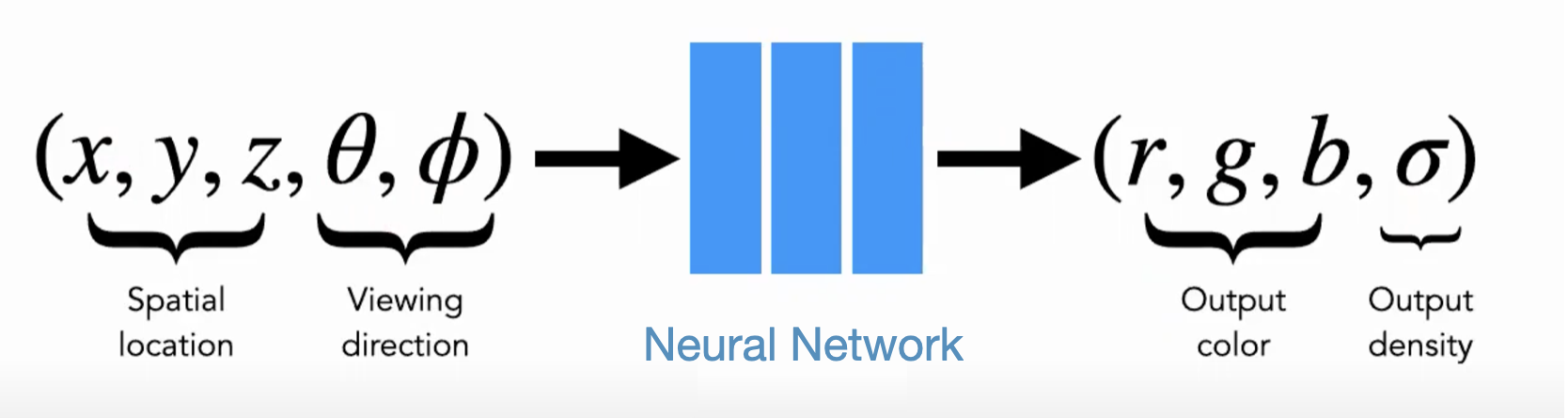
Since we’re just doing a vector to vector mapping, the typical architecture used for a NeRF is a vanilla neural network, often referred to as a Multilayer Perceptron, or MLP. The standard architecture introduced in the NeRF paper uses 8 hidden layers with 1024 neurons in each layer. In some cases, the object at a location may appear differently depending on the direction it is viewed from. To account for this, NeRFs also condition the network on a specific viewing direction specified as angles. This adds another two inputs to the neural network, bringing the total to five.

Note that a NeRF and its parameters are unique to a single object. This is somewhat atypical in machine learning where we want to use a dataset to learn how to make predictions on new and unseen data. Here, you can think of an observed view of an object as a single datapoint and observe that by fitting our NeRF to the object using these views we’re able to make predictions about new and unseen viewing directions. This entire approach works because shapes tend to have discernible patterns and neural networks are effective pattern recognition tools.

Later on we’ll discuss in depth the procedure for training NeRFs and actually finding the “right” parameters $\Theta$, but for now we can assume that we have these parameters on hand and get better acquainted with NeRFs.

Positional Encoding

As mentioned earlier, the network for our NeRF is reliant upon the $xyz$ coordinate values to represent the radiance field. Its performance is therefore entirely depend on its ability to discriminate within this input feature space which makes it somewhat unsurprising that one of the key breakthroughs in getting NeRFs to work was a feature engineering trick aimed at these spatial coordinates.

What the authors of the original NeRF paper found was that instead of representing a coordinate value as a single scalar, they could get more performant features by instead mapping the coordinate to a higher-dimensional vector. This mapping is chosen such that the vector can still uniquely identify the scalar input while also gaining additional properties that make for a more neural-network-friendly representation. The specifics of this can be a bit tricky to understand so I’ll try to give you a close look at the mathematical definitions along with some intuition in case the math doesn’t make sense. I’ll also further discourage you from closing this tab by noting that positional encodings are an important building block in transformers (though for different reasons) so by wrapping your head around this you’ll be knocking out two birds with one stone.

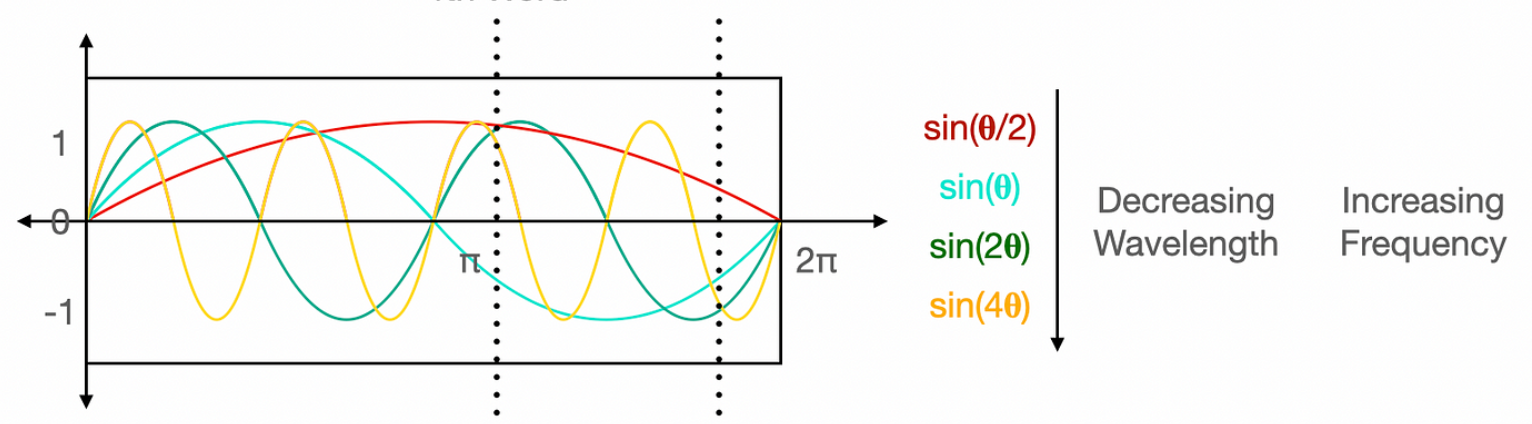
The basic idea is that if you have a bunch of sine and cosine functions at different frequencies and you evaluate all of these functions at the same input value $p$ then by looking at the set of outputs you should be able to recover $p$. For instance, looking at the graph of different curves, we can see that any vertical slice we take is going to intersect the curves in wildly different locations due to the rapidly divergent behavior of each curve. Because of this, we can represent a location on the x-axis of the graph using this sequence of sines: $sin(\frac{p}{2}),sin(p),sin(2p),sin(4p)$ and by doing so we’ll get a unique identifier of that location. By extending this and adding cosines, we can define a function $\alpha: \mathbb{R}\rightarrow \mathbb{R}^{2L}$

Now that we’ve established that we’re not losing any information by replacing $p$ with $\alpha(p)$ the obvious question arises: What could we possibly be gaining by doing this? If our positional encoding just represents the same information as a scalar, but in a more convoluted and annoying form, then how are we not just taking a clear step backward? In fact, this encoding seems to runs contrary to the generally desirable goal of distilling and compressing information into a minimally complex form.

The answer here mainly boils down to the fact that it helps NeRFs capture high-frequency patterns in spatial data. Because $\alpha$ makes use of waves of varying frequencies, some (but not all) of its component functions change very rapidly with respect to their input. This is essential for our NeRF to capture the fine-grained detail of in certain objects. Of course, not all the patterns we wish to capture are of a high frequency and we also want it to be easy for our network to smoothly trace less steep contours. This formulation allows a best-of-both-worlds solution as it makes NeRFs sensitive to small changes in coordinate space while also permitting them to not be sensitive to small changes in coordinate space when the downstream MLP decides that’s what’s needed. How flexible!

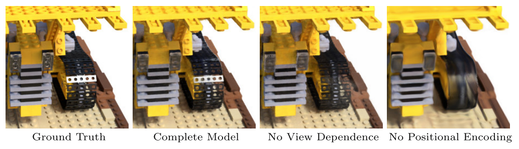
Of course, just an MLP by itself is capable of representing both high and low frequency functions (let’s not contradict the UAT) it’s just that neural networks are kind of lazy and have a tendency to find optima which have low-frequency solutions. Using these spatial encodings adds a bias towards proper shape representation, leading to better performance with fewer parameters. Below you can see an ablation from the original NeRF paper which shows the result of fitting a NeRF to a ground-truth 3D model with the removal of view-dependence (those additional $\theta,\phi$ inputs) and positional embedding. Without positional embedding, the fine-grained details are reduced to a blurry approximation.

Nowadays, many applications use a slightly more sophisticated form of spatial embedding introduced in the Mip-NeRF paper or leverage a clever data structure to store explicit embeddings like in NVIDIA’s Instant-NGP. However, most solutions are closely related to the ideas presented here and and are meant to provide application-specific improvements.

Rendering an Image with NeRFs

Now that we have a solid understanding of how a NeRF produces its radiance outputs, let’s look at how to apply $f_{\Theta}$ to obtain image observations. In this section we’ll take a closer look at how color and occupancy values are used to generate images, so we’ll also the terms $r_{\Theta}$ and $c_{\Theta}$ to separetely denote their respective functions.

Raytracing

For simplicity, we can avoid thinking about rendering an entire image and just focus on how to capture a single pixel. To do this, you can build a mental picture of what goes in your camera to capture a pixel’s worth of color when you point it at an object and click the button. Put plainly, your camera emits a ray of light from the pixel location which retrieves the pixel value. This ray shoots forward in a straight line toward the object until it makes contact with its surface. The pixel color is then determined by the RGB value at this infinitesimal point of contact.

To imbue this intuition with some mathematical rigor, we can define our ray as a function $\bf{r}(t)$ that maps a time value to the 3D position the ray gets to at that time. When “shooting” a scene from a given angle, it’s trivial to trace this ray’s linear trip through space. Using our NeRF parameters also enables us compute the color $c_{\Theta}(\bf{r}(t))$ and opacity $\sigma_{\Theta}(\bf{r}(t))$ that our ray will encounter at any time value.

Note: For a more detailed treatment of raytracing (also called raymarching), you can see this interactive demonstration

Neural Rendering

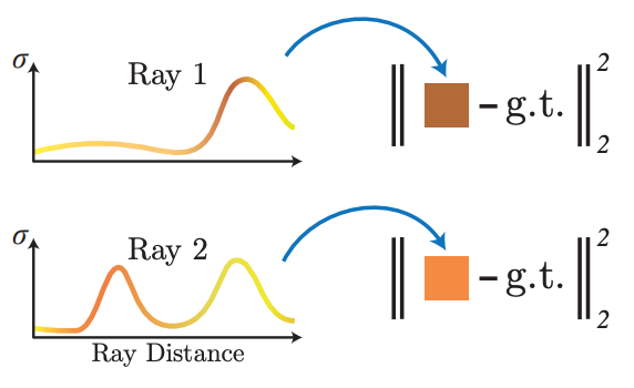
These are pretty much all the components required for us to get to a formula to compute the actual pixel value for a ray that is shot through our NeRF scene. The only further caveat is that the above description in which the ray simply “makes contact” with the object assumes that opacity is a binary value so the ray travels freely before all at once hitting something solid. In actuality, our operating definition of opacity only restricted it between $0$ and $1$. This was intentional, as using a continuous value allows us to represent partially opaque objects and makes the mapping from scene to image differentiable. In this setting, instead of being stopped abrutly it’s more like our ray gets gradually worn down as it encounters non-opaque regions. This lessens the effect of the colors it reaches later which are only partially visible. With that in mind, we can define the pixel color $C(r,\Theta)$ by integrating over the ray’s path as it accumulates colors it encounters in high-opacity regions.

The second formula for $T(t)$ expresses how much of the ray is left at that time and hasn’t already been blocked out. Once the value of $T(t)$ becomes very close to $0$ we can stop our raytracing as the remaining domain will have a negligible effect on the overall color. It is this stopping criterion which allows us to avoid querying irrelevant regions.

In practice, these integrals are approximated using a finite sum, which gives us some easily computable color $\hat{C}(r,\theta) \approx C(r,\theta)$. It’s also standard to include some cutoff point for the upper bound of the integral as some rays never make contact with our scene, leaving the corresponding pixel to be black. If you understand this procedure for obtaining the color of a single pixel, then it’s then pretty trivial to scale up to computing to an entire image as this procedure can be easily parallelized across a GPU.

Note: In practice NeRFs employ a technique called hierarchical volume sampling to get better efficiency when breaking integral computations into finite sums. I’ve left this out since it’s not essential to understanding NeRFs but the interesed reader can find a detailed description in the NeRF paper

Training A NeRF

Up until now we’ve just assumed that $\Theta$ has been chosen so that it correctly represents the radiance field for the scene being portrayed. Now we move to a more realistic case in which we make no assumptions about the quality of $f_{\Theta}$ and take it upon ourselves to adjust the parameters in a sensible direction. To accomplish this we’ll derive loss functions that are both tractable (can be computed efficiently) and differentiable (have well-defined gradients).

3D Reconstruction

Since we wish to impose some idea of “correctness”, we require a ground-truth for comparison purposes. This supervision is almost always in image-space as this is the most common way to observe 3D data. Lucky for us, we know how to use our NeRF parameters to render our shape into image space, getting pixel values $\hat{C} (\bf{r},\Theta)$.

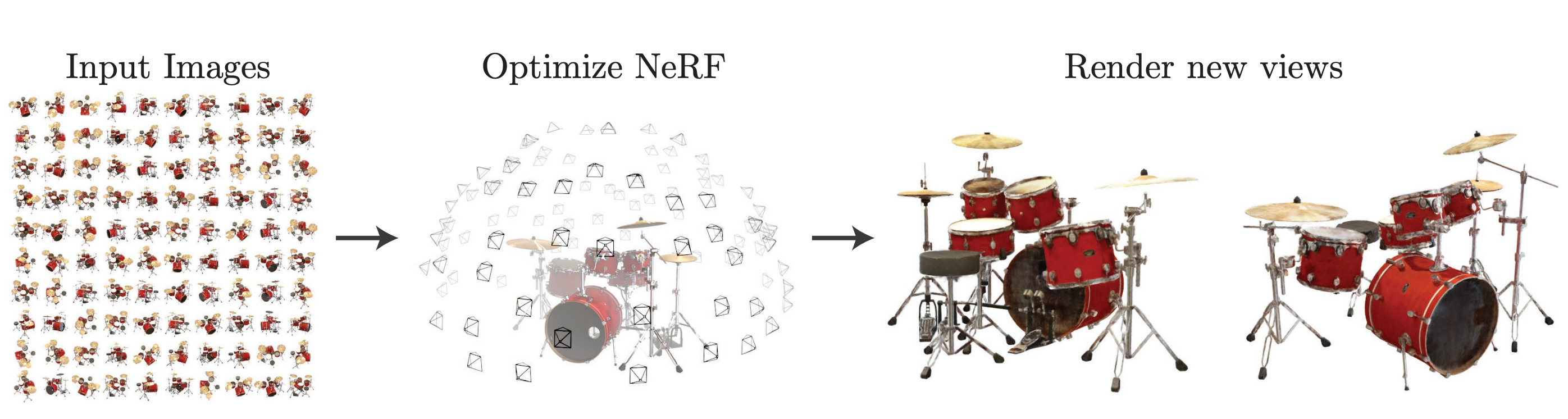
We can use this to perform 3D reconstruction where we are given a set of images which depict a shape or scene and want to optimize our shape representation so that it could plausibly produce those images. As long as we know the camera parameters used to take the photos, we can see each pixel of these images as a ground truth value $C_{gt}(\bf{r})$ that tell us the correct value for a specific ray. This correct value is the pixel value we would hope to get when we shoot that same ray through our NeRF. To turn this into a training loss, we randomly sample a batch of rays $\mathcal{R}$ from our image set and find the difference between the ground truth and what we get from our NeRF.

Computing this is fairly straightforward and because our mapping from $\Theta$ to $\hat{C}(\bf{r},\Theta)$ is constructed to be fully differentiable, the loss can be backpropagated into our network parameters. Below you can see samples of how NeRFs evolve over the training procedure. I think this does a good job of illustrating why we need our opacity values to be continuous, even when we’re only representing solid objects, as the true scenes emerge from clouds of partial opacity.

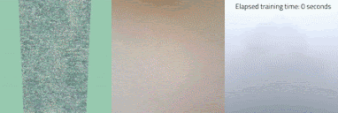
This .gif doesn’t seem to work all the time, so if it freezes for you the source is here

To make this work in practice, the original NeRF methodology uses 4096 rays per batch and samples 128 points along each ray to get $\hat{C}(\bf{r},\Theta)$. Repeating this until convergence takes between 100k and 300k iterations.

Text-Conditioned Training

As I said before, 3D reconstruction is the canonical setup for training NeRFs but it’s just one of many settings in which NeRFs can be used. To give you an additional example, I’ll briefly touch on how this training can be extended to training a text-conditioned NeRF. Here, we have some textual description $t$ which specifies a shape we’d like for our NeRF to represent.

We can actually define a fairly simple loss function for this goal and remarkably, this loss will still operate entirely in the image space. This is because we can take advantage of the shared image-text powers of OpenAI’s CLIP. Without delving too much into how CLIP is trained, it computes vector embeddings of both images and text so that these embeddings retain their semantic information. This means that for some image $\mathcal{I}$ which depicts a toaster and the text string “toaster” we can expect the inner product $\left<\text{CLIP}(I),\text{CLIP}(“toaster”)\right>$ to have a high value indicating their semantic similarity.

Applying this to our NeRF, we can use CLIP similarity as a training objective in image space. Instead of rendering individual rays from $f_{\Theta}$, we can instead render an entire image $\mathcal{I}$ at once and then compute the image’s semantic similarity with our text prompt $t$. This naturally yields the following loss function:

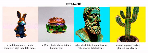
This approach was first introduced in Google’s Dreamfields paper a few years ago and while further improvements have been proposed by others, the sheer simplicity of this still amazes me. I already included some samples of text-to-3D outputs but you can click the hyperlink to check out a more extensive gallery if you wish or even look at the follow-up works Dreamfusion and MVDream

NeRF Descendants

While I’ve mostly stuck to the NeRF formulation introduced in the original NeRF paper by Mildenhall et al. I’ve also included some notes about architectural changes introduced in later works where relevant. Here I want to give a more in-depth look at some of the more recent works which have been inspired by NeRFs.

PixelNeRF

One drawback of NeRFs which I noted earlier is that they are single-use, meaning that they only fit a network to one scene and need to be completely retrained if you want to use them for something else. To address this, PixelNeRF proposed a few-shot architecture which produces 3D representations from images of new shapes without requiring any further optimization.

To do this, PixelNeRF conditions the NeRF MLP on an additional input $z$, which is a latent vector representation of a specific 3D shape. So long as we have access to this latent vector we can produce the RGB and opacity values for any shape by computing $f_{\Theta}(x,y,z,\theta,\phi,z)$. To learn parameters $\Theta$ which will apply to all shapes, they do standard NeRF training over a vast dataset of different shapes.

Of course, we’d like to be able to use this generalized NeRF for any shape we have a set of images of rather than requiring this latent vector representation $z$. To fix this, PixelNeRF also trains an encoder model $h_{\Omega}$ to map from images to low-dimensional shape representations. This is trained jointly with $f_{\Theta}$ so that both of these networks are able to generalize over a diverse distribution of shapes.

The result is a very useful tool that only requires a few images (as few as one!) of an object to generate a detailed 3D representation. To use PixelNeRF on a novel object, the first step is to feed the ground-truth images into the encoder $h_{\Omega}$ to get an embedding of the object $z$. Then by conditioning $f_{\Theta}$ on $z$, it can be used to render novel views of the object. This doesn’t require any changes to $\Theta$ or learning of any kind as $z$ alone captures all the object-specific information needed for 3D reconstruction!

Gaussian Splatting

Despite what I said early on about explicit methods and their drawbacks, they’re actually having a real moment right now with the advent of something called Gaussian Splatting. The core idea of Gaussian Splatting is to adopt the overall scene representation framework of NeRFs, but to fit the radiance field using a model that isn’t a neural network. Instead, they use a gaussian mixture model with a fixed number of gaussian components which explicitly represent the scene at different locations.

While their explicit nature still leaves them with a higher memory overhead than NeRFs they are much faster to render once learned. In the case of NeRFs, we have to start from the viewing direction and raymarch toward the shape because we don’t have explicit knowledge of where the shape is. This wastes a lot of time and compute on empty space. For Guassian Splatting, using a discrete representation structure means only having to check which gaussians will be visible from a given angle and render (or “splat”) them outward toward the viewing direction.

This acceleration of inference capabilities is significant as it allows for “real-time” rendering, so that a user can interact with a 3D scene and have it rendered for them so quickly that the delay is not noticeable. This opens up all sorts of applications in synthesized videos and interactive scenes which were not previously possible with NeRFs.

Wrapping Up

So in this post we’ve seen the benefits of using NeRFs to implicitly represent 3D scenes, gotten a good grasp of the technical details that enable their performance, and demonstrated how their flexibility allows for different types of training. If this sparked your interest, there’s no shortage of followup works in this area that I’d highly encourage you to check out! This is a fast-moving area with lots of progress ongoing and there’s no telling what the future holds for 3D machine learning.